System for the automated classification of white blood cells (leukocytes). Input is a WBC image and the output is the class of the given image.

You can download the LISC (Leukocyte Images for Segmentation and Classification) database from the following link: http://users.cecs.anu.edu.au/~hrezatofighi/Data/Leukocyte%20Data.htm

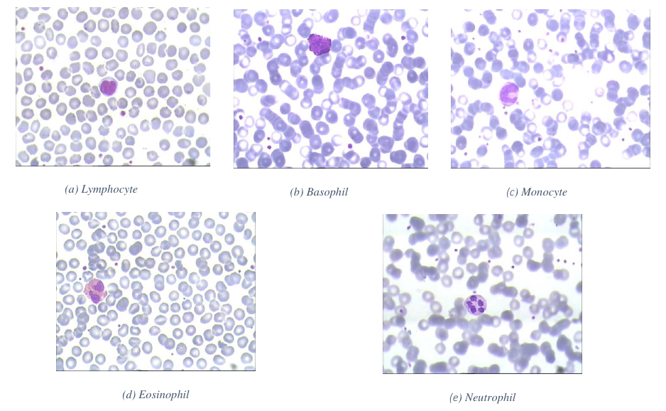
An example of each of the five classes of white blood cell is shown in the following figure:

Phase 1: Segmentation

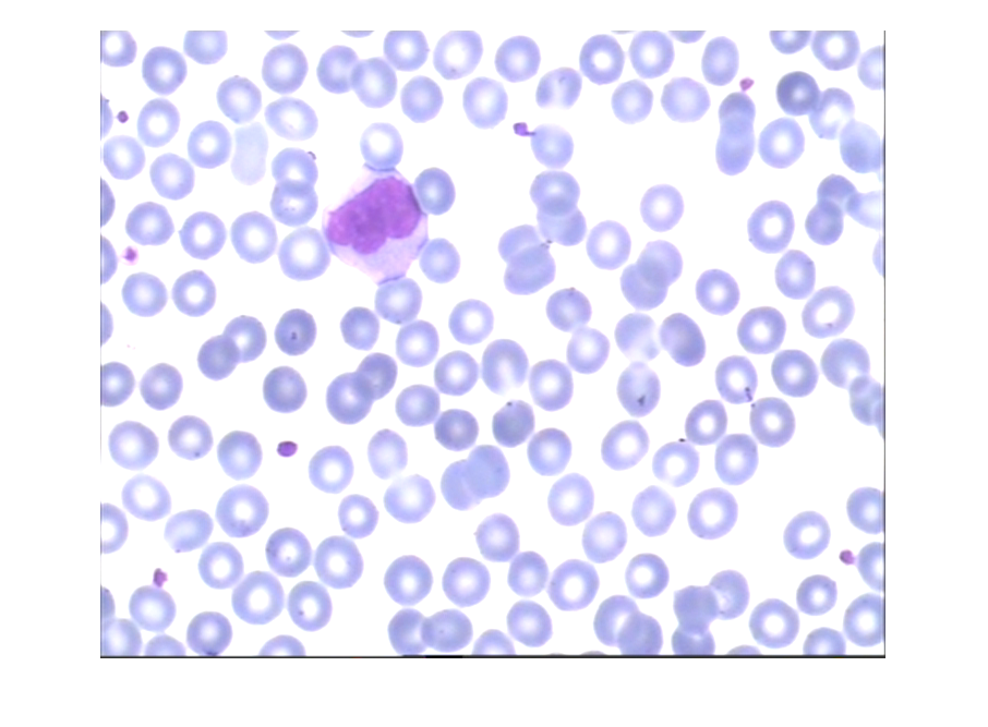
Load a random specimen as HSV#

Different color spaces has been tested (RGB, LAB, LIN) and found HSV is most suitable for the given task.

img = rgb2hsv(imread('specimen.bmp'));
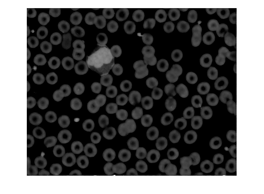
% Extract the second layer
layer = img(:, :, 2);
imshow(layer);

Original RGB Sample	HSV’s saturation layer

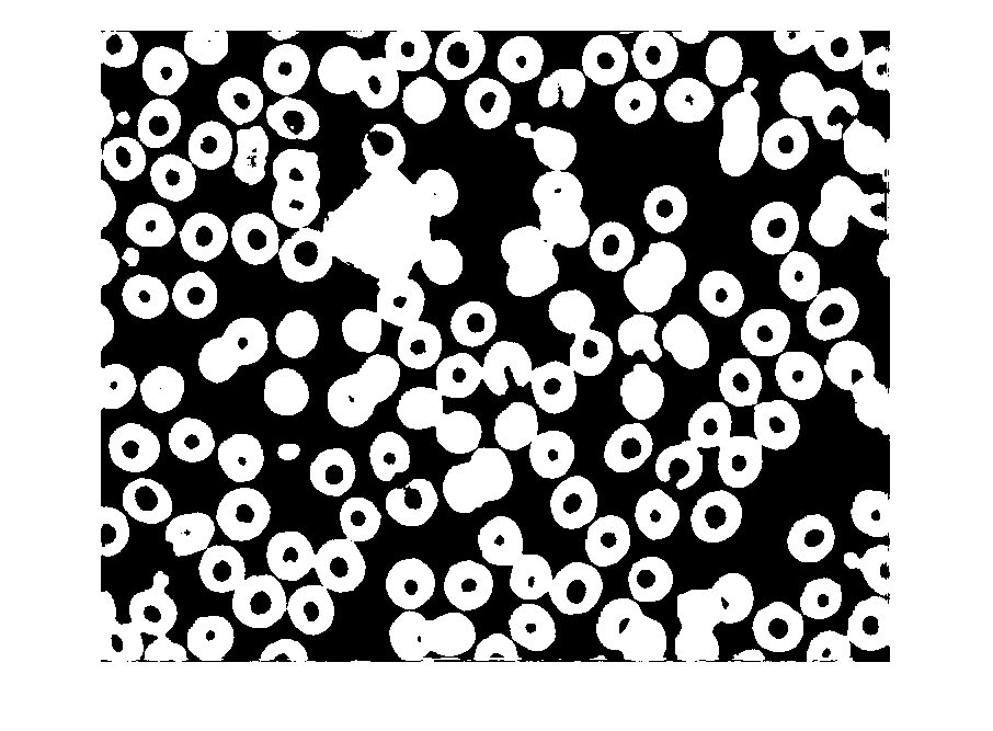
Isolate nucleus#

The process mainly involved carefully incrementing the threshold until an optimal segment has been found.

Here is the result of a careful iterative process over a large sample to extract the nucleus.

nucleusThreshold = 0.3686;
p1 = layer > nucleusThreshold;
imshow(p1);

Prune nucleus#

Small unwanted artifacts can be removed by an open mask with a disk structural element of size 8.

se = strel('disk', 8);
p1 = imopen(p1, se);

Isolate surrounding fluid#

The surrounding fluid is essential in identifying variations of whiteblood cells.

Similar process of isolating the nucleus has been used to isolate the fluid.

fluidThreshold = 0.0980;
p2 = layer > fluidThreshold;
imshow(p2);

Prune fluid#

Same as nucleus, unwanted artifacts can be removed by an open mask with a disk structural element but with a size 28.

se = strel('disk', 28);
p2 = imopen(p2, se);
imshow(p2);

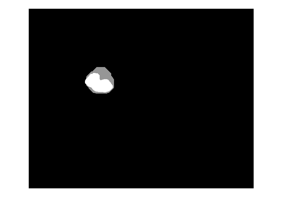
Merge nucleus with fluid#

Here the fluid is given a more distinguished color (used 150 grey) then added to the nucleus.

p1 = im2uint8(p1);
p2 = im2uint8(p2);
p2(p2 == 255) = 150; % distinguish fluid from nucleus
imshow(p1 + p2);     % combine components

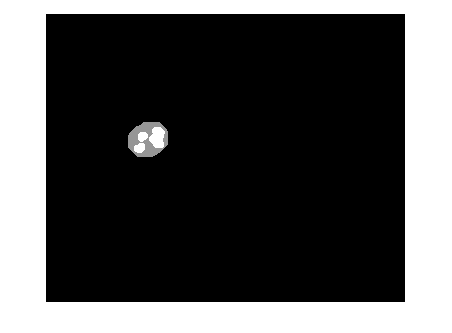
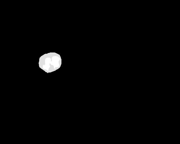
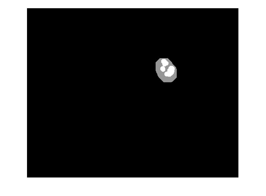
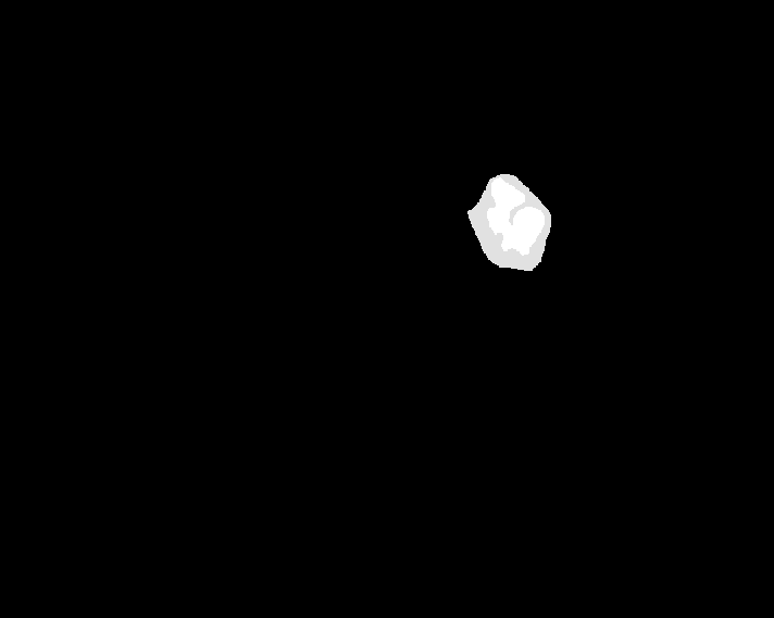
Examples#

SAMPLE_SIZE = 6;
for i=1:SAMPLE_SIZE
    res = imread('samples/' + string(i) + '_res.png');
    ref = imread('samples/' + string(i) + '_expert.bmp');
    % figure, imshowpair(res, ref, 'montage');
    subplot(1, 2, 1), imshow(res);
    subplot(1, 2, 2), imshow(ref);
    figure;
end

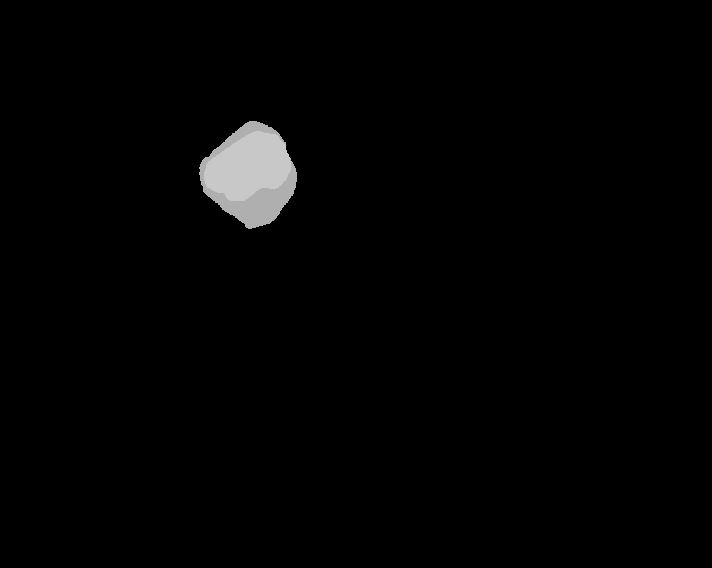
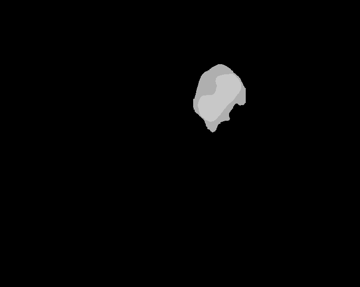
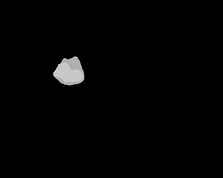
Segmenter	Ground Truth

Phase 2: Feature Extraction

Deep Learning is a machine learning technique that can learn useful representations and features directly from images. A CNN learn these features automatically from images from generic low level features like edge and corners all the way to specific problem features.

Deep Learning algorithms not only perform classification but also learn to extract features directly from image, thereby eliminate the need for manual feature extraction.

Instead of training a CNN from scratch, we use a pre-trained CNN model (VGG-19) as an automatic feature extract known as Transfer Learning.

VGG-19 has been trained on over a million images and can classify images into 1000 object categories (such as keyboard, coffee mug, pencil, and many animals).

The network has learned rich feature representations for a wide range of images. The network takes an image as input and outputs a label for the object in the image together with the probabilities for each of the object categories.

Here a demonstration on how to fine-tune a pre-trained VGG-19 CNN to perform classification on LISC image database.

Training Model#

%% Load Dataset
dsTrain = imageDatastore('train', 'IncludeSubfolders', true, ...
                                  'LabelSource', 'foldernames');
dsValidate = imageDatastore('validate', 'IncludeSubfolders', true, ...
                                     'LabelSource', 'foldernames');
%% Resize Dataset
augTrain = augmentedImageDatastore([224 224], dsTrain);
augValidate = augmentedImageDatastore([224 224], dsValidate);
%% Load VGG-19 network
net = vgg19();
analyzeNetwork(net)
%% Replace last layers
layersTransfer = net.Layers(1:end-3);
numClasses = numel(categories(dsTrain.Labels))

layers = [
    layersTransfer
    fullyConnectedLayer(numClasses,'WeightLearnRateFactor', 20, ...
                                   'BiasLearnRateFactor', 20)
    softmaxLayer
    classificationLayer];

%% Network options
options = trainingOptions('sgdm', ...
                        'MiniBatchSize',10, ...
                        'MaxEpochs',6, ...
                        'InitialLearnRate',1e-4, ...
                        'Shuffle','every-epoch', ...
                        'ValidationData',augValidate, ...
                        'ValidationFrequency',3, ...
                        'Verbose',false, ...
                        'Plots','training-progress');
%% Train Network
vgg19LISC = trainNetwork(augTrain, layers, options);

Layers Details#

Layer Number	Name	Type	Description
1	input	Image Input	224x224x3 images with ‘zerocenter’ normalization
2	conv1_1	Convolution	64 3x3x3 convolutions with stride [1 1] and padding [1 1 1 1]
3	relu1_1	ReLU	ReLU
4	conv1_2	Convolution	64 3x3x64 convolutions with stride [1 1] and padding [1 1 1 1]
5	relu1_2	ReLU	ReLU
6	pool1	Max Pooling	2x2 max pooling with stride [2 2] and padding [0 0 0 0]
7	conv2_1	Convolution	128 3x3x64 convolutions with stride [1 1] and padding [1 1 1 1]
8	relu2_1	ReLU	ReLU
9	conv2_2	Convolution	128 3x3x128 convolutions with stride [1 1] and padding [1 1 1 1]
10	relu2_2	ReLU	ReLU
11	pool2	Max Pooling	2x2 max pooling with stride [2 2] and padding [0 0 0 0]
12	conv3_1	Convolution	256 3x3x128 convolutions with stride [1 1] and padding [1 1 1 1]
13	relu3_1	ReLU	ReLU
14	conv3_2	Convolution	256 3x3x256 convolutions with stride [1 1] and padding [1 1 1 1]
15	relu3_2	ReLU	ReLU
16	conv3_3	Convolution	256 3x3x256 convolutions with stride [1 1] and padding [1 1 1 1]
17	relu3_3	ReLU	ReLU
18	conv3_4	Convolution	256 3x3x256 convolutions with stride [1 1] and padding [1 1 1 1]
19	relu3_4	ReLU	ReLU
20	pool3	Max Pooling	2x2 max pooling with stride [2 2] and padding [0 0 0 0]
21	conv4_1	Convolution	512 3x3x256 convolutions with stride [1 1] and padding [1 1 1 1]
22	relu4_1	ReLU	ReLU
23	conv4_2	Convolution	512 3x3x512 convolutions with stride [1 1] and padding [1 1 1 1]
24	relu4_2	ReLU	ReLU
25	conv4_3	Convolution	512 3x3x512 convolutions with stride [1 1] and padding [1 1 1 1]
26	relu4_3	ReLU	ReLU
27	conv4_4	Convolution	512 3x3x512 convolutions with stride [1 1] and padding [1 1 1 1]
28	relu4_4	ReLU	ReLU
29	pool4	Max Pooling	2x2 max pooling with stride [2 2] and padding [0 0 0 0]
30	conv5_1	Convolution	512 3x3x512 convolutions with stride [1 1] and padding [1 1 1 1]
31	relu5_1	ReLU	ReLU
32	conv5_2	Convolution	512 3x3x512 convolutions with stride [1 1] and padding [1 1 1 1]
33	relu5_2	ReLU	ReLU
34	conv5_3	Convolution	512 3x3x512 convolutions with stride [1 1] and padding [1 1 1 1]
35	relu5_3	ReLU	ReLU
36	conv5_4	Convolution	512 3x3x512 convolutions with stride [1 1] and padding [1 1 1 1]
37	relu5_4	ReLU	ReLU
38	pool5	Max Pooling	2x2 max pooling with stride [2 2] and padding [0 0 0 0]
39	fc6	Fully Connected	4096 fully connected layer
40	relu6	ReLU	ReLU
41	drop6	Dropout	50% dropout
42	fc7	Fully Connected	4096 fully connected layer
43	relu7	ReLU	ReLU
44	drop7	Dropout	50% dropout
45	fc	Fully Connected	5 fully connected layer
46	softmax	Softmax	softmax
47	classoutput	Classification Output	crossentropyex with ‘baso’ and 4 other classes

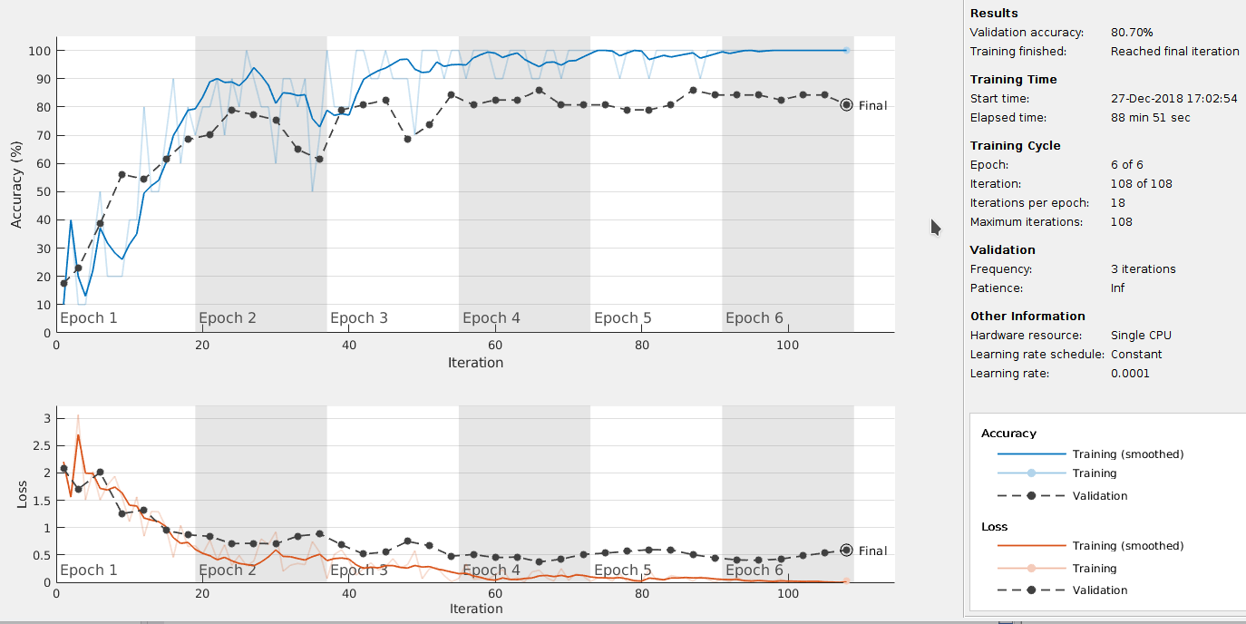
Training Result#

Using Model#

%% Load Existing Model
load('vgg19LISC.mat');

sample = imread('sample');
sample = imresize(sample, [224 224]); %% Dont forget to resize sample

Repository#

Code, training and validating datasets used are available here.